PCA of gene expression in CTCs from NSG-CDX-BR16 mice
Francesc Castro-Giner
2022-02-23
Last updated: 2022-05-12
Checks: 7 0
Knit directory:
diamantopoulou-ctc-dynamics/
This reproducible R Markdown analysis was created with workflowr (version 1.6.2). The Checks tab describes the reproducibility checks that were applied when the results were created. The Past versions tab lists the development history.
Great! Since the R Markdown file has been committed to the Git repository, you know the exact version of the code that produced these results.
Great job! The global environment was empty. Objects defined in the global environment can affect the analysis in your R Markdown file in unknown ways. For reproduciblity it’s best to always run the code in an empty environment.
The command set.seed(20220425) was run prior to running
the code in the R Markdown file. Setting a seed ensures that any results
that rely on randomness, e.g. subsampling or permutations, are
reproducible.
Great job! Recording the operating system, R version, and package versions is critical for reproducibility.
Nice! There were no cached chunks for this analysis, so you can be confident that you successfully produced the results during this run.
Great job! Using relative paths to the files within your workflowr project makes it easier to run your code on other machines.
Great! You are using Git for version control. Tracking code development and connecting the code version to the results is critical for reproducibility.
The results in this page were generated with repository version a747daf. See the Past versions tab to see a history of the changes made to the R Markdown and HTML files.
Note that you need to be careful to ensure that all relevant files for
the analysis have been committed to Git prior to generating the results
(you can use wflow_publish or
wflow_git_commit). workflowr only checks the R Markdown
file, but you know if there are other scripts or data files that it
depends on. Below is the status of the Git repository when the results
were generated:
Ignored files:
    Ignored:    .Rhistory
    Ignored:    .Rproj.user/

Untracked files:
    Untracked:  analysis/0_differential_expression_gsea_gsva.md
    Untracked:  analysis/about.md
    Untracked:  analysis/br16_dge.md
    Untracked:  analysis/br16_pca.md
    Untracked:  analysis/core_gene_sets.md
    Untracked:  analysis/gsea_across_models.md
    Untracked:  analysis/index.md
    Untracked:  analysis/license.md
    Untracked:  analysis/patients_ctc_counts_distribution.md
    Untracked:  data/differential_expression/
    Untracked:  data/patients/
    Untracked:  data/resources/
    Untracked:  data/sce/
Note that any generated files, e.g. HTML, png, CSS, etc., are not included in this status report because it is ok for generated content to have uncommitted changes.
These are the previous versions of the repository in which changes were
made to the R Markdown (analysis/br16_dge.Rmd) and HTML
(docs/br16_dge.html) files. If you’ve configured a remote
Git repository (see ?wflow_git_remote), click on the
hyperlinks in the table below to view the files as they were in that
past version.
| File | Version | Author | Date | Message |
|---|---|---|---|---|
| html | 1fc87b5 | fcg-bio | 2022-05-10 | Build site. |
| html | 8fb5513 | fcg-bio | 2022-05-10 | Build site. |
| html | 8acaa64 | fcg-bio | 2022-04-26 | Build site. |
| Rmd | 545ee28 | fcg-bio | 2022-04-26 | release v1.0 |
| html | 74b1891 | fcg-bio | 2022-04-26 | Build site. |
| html | c0865c6 | fcg-bio | 2022-04-26 | Build site. |
| html | a136590 | fcg-bio | 2022-04-26 | Build site. |
| html | bfb622b | fcg-bio | 2022-04-26 | Build site. |
| html | 1006c84 | fcg-bio | 2022-04-26 | Build site. |
| Rmd | 0ded9f5 | fcg-bio | 2022-04-26 | added final code |
Load libraries, additional functions and data
Setup environment
knitr::opts_chunk$set(results='asis', echo=TRUE, message=FALSE, warning=FALSE, error=FALSE, fig.align = 'center', fig.width = 3.5, fig.asp = 0.618, dpi = 600, dev = c("png", "pdf"), fig.showtext = TRUE)

options(stringsAsFactors = FALSE)
Load packages
library(tidyverse)
library(showtext)
library(scater)
library(ComplexHeatmap)
library(circlize)
library(RColorBrewer)
library(DT)
Set font family for figures
font_add("Helvetica", "./configuration/fonts/Helvetica.ttc")
showtext_auto()
Load ggplot theme
source("./configuration/rmarkdown/ggplot_theme.R")Load color palettes
source("./configuration/rmarkdown/color_palettes.R")Load SingleCellExpression data
use_sce <- readRDS(file.path(params$sce_dir, 'sce_br16.rds'))Load results from differential gene expression analyses
dge_all <- readRDS(file.path(params$dge_dir, 'br16', 'dge_edgeR_QLF_robust.rds'))
dge_cluster_g <- readRDS(file.path(params$dge_dir,'br16-ctc_cluster_and_wbc', 'dge_edgeR_QLF_robust.rds'))
dge_single <- readRDS(file.path(params$dge_dir,'br16-ctc_single', 'dge_edgeR_QLF_robust.rds'))
Genes differentially expressed in CTCs of NSG-CDX-BR16
Genes differentially expressed in CTCs of NSG-CDX-BR16 mice during the rest phase versus active phase. Table listing the differentially expressed genes comparing CTCs obtained in the rest phase (n = 65) versus the active phase (n = 73) of NSG-CDX-BR16 mice. All genes evaluated are included in the table (n = 12,261). Fold-change and P values were computed with the quasi-likelihood (QL) approach from edgeR using robust dispersion estimates. For fold-change calculation, active phase samples were used in the denominator.
dge_all$results %>%
dplyr::select(gene_name, gene_type, logFC, logCPM, PValue, FDR, description) %>%
rownames_to_column('Ensemble ID') %>%
mutate(
logFC = round(logFC, 2),
logCPM = round(logCPM, 2),
PValue = format.pval(PValue, digits = 2),
FDR = format.pval(FDR, digits = 2),
description = gsub(" \\[.*\\]", "", description)
) %>%
dplyr::rename(
`Gene name` = gene_name,
`Gene type` = gene_type
) %>%
datatable(.,
rownames = FALSE,
filter = 'top',
caption = 'Genes differentially expressed in CTCs of NSG-CDX-BR16 mice during the rest phase versus active phase.',
extensions = 'Buttons',
options = list(
dom = 'Blfrtip',
buttons = c('csv', 'excel'),
title = paste('', params$prefix)
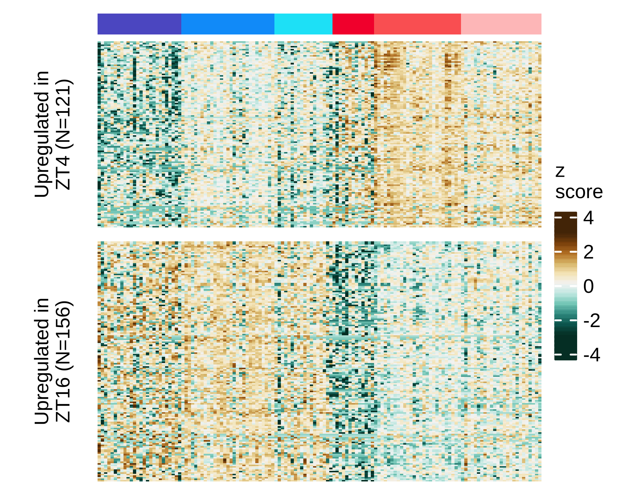
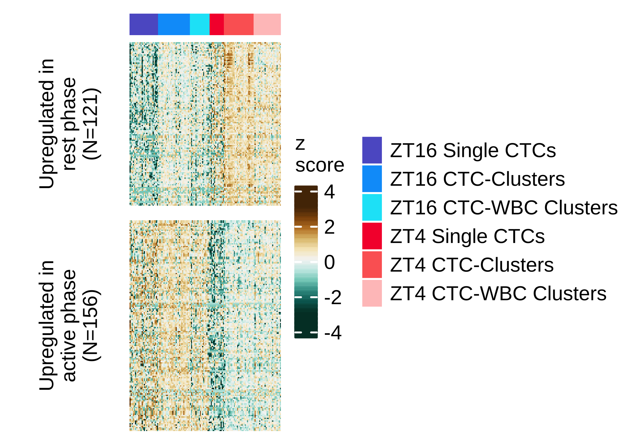
))Heatmap differential expression NSG-CDX-BR16 mice
Heatmap showing expression levels (row scaled z-scores using normalized counts) of differentially-expressed genes between rest and active phase (absolute log2 fold change ≥ 0.5 and FDR ≤ 0.05) in CTCs from NSG-BR16-CDX mice.
dge <- dge_all
use_genes <- dge$results %>% filter(FDR <= 0.05 & abs(logFC) >= 0.5) %>% collect %>% .[['feature']]
use_genes_name <- rowData(use_sce[use_genes,]) %>% data.frame %>% collect %>% .[['gene_name']]
n_up <- dge$results %>% filter(FDR <= 0.05 & logFC >= 0.5) %>% nrow
n_down <- dge$results %>% filter(FDR <= 0.05 & logFC <= -0.5) %>% nrow
expr_values <- logcounts(use_sce[use_genes,])
heat_values <- t(apply(expr_values, 1, scale, center = TRUE, scale = TRUE)) # Z-score
rownames(heat_values) <- use_genes_name
colnames(heat_values) <- colnames(expr_values)

coldata_ord <- colData(use_sce) %>% data.frame %>% arrange(zt_sample_type_legend)
heat_values <- heat_values[,coldata_ord$sample_alias]

ha_top <- HeatmapAnnotation(
  show_legend = FALSE,
  `CTC type` = coldata_ord$zt_sample_type_legend,
  col = list(`CTC type` = zt_sample_type_legend_palette),
  annotation_legend_param = list(
    title = NULL,
    title_gp = gpar(fontsize = 8),
    labels_gp = gpar(col = "black", fontsize = 8),
    grid_width = unit(3, "mm")
    ),
  show_annotation_name = FALSE,
  simple_anno_size = unit(3, "mm")
  )

zlim <- c(-3, 3)
heat_values[heat_values < zlim[1]] <- zlim[1]
heat_values[heat_values > zlim[2]] <- zlim[2]

col_fun <-  colorRamp2(seq(zlim[1], zlim[2], length.out = 11), rev(brewer.pal(n = 11, name ="BrBG")))

Heatmap(
  heat_values,
  name = 'z\nscore',
  col =  col_fun,
  row_split = 2,
  row_gap = unit(2, "mm"),
  cluster_columns = FALSE,
  column_title = NULL,
  row_title = NULL,
  show_column_dend = FALSE,
  show_column_names = FALSE,
  show_row_dend = FALSE,
  show_row_names = FALSE,
  top_annotation = ha_top,
  left_annotation = rowAnnotation(foo = anno_block(
        labels = c(
          paste0("Upregulated in\nZT4 (N=", n_up, ")"),
          paste0("Upregulated in\nZT16 (N=", n_down, ")")
        ),
        labels_gp = gpar(col = "black", fontsize = 8),
        gp = gpar(lwd = 0, lty = 0)
        )
  ),
  heatmap_legend_param = list(
    title_gp = gpar(fontsize = 8),
    labels_gp = gpar(fontsize = 8),
    grid_width = unit(3, "mm")
    )
)
| Version | Author | Date |
|---|---|---|
| 1006c84 | fcg-bio | 2022-04-26 |
use_genes <- dge$results %>% filter(FDR <= 0.05 & abs(logFC) >= 0.5) %>% collect %>% .[['feature']]
use_genes_name <- rowData(use_sce[use_genes,]) %>% data.frame %>% collect %>% .[['gene_name']]
n_up <- dge$results %>% filter(FDR <= 0.05 & logFC >= 0.5) %>% nrow
n_down <- dge$results %>% filter(FDR <= 0.05 & logFC <= -0.5) %>% nrow
expr_values <- logcounts(use_sce[use_genes,])
heat_values <- t(apply(expr_values, 1, scale, center = TRUE, scale = TRUE)) # Z-score
rownames(heat_values) <- use_genes_name
colnames(heat_values) <- colnames(expr_values)

coldata_ord <- colData(use_sce) %>% data.frame %>% arrange(zt_sample_type_legend)
heat_values <- heat_values[,coldata_ord$sample_alias]

ha_top <- HeatmapAnnotation(
  show_legend = TRUE,
  `CTC type` = coldata_ord$zt_sample_type_legend,
  col = list(`CTC type` = zt_sample_type_legend_palette),
  annotation_legend_param = list(
    title = NULL,
    title_gp = gpar(fontsize = 8),
    labels_gp = gpar(col = "black", fontsize = 8),
    grid_width = unit(3, "mm")
    ),
  show_annotation_name = FALSE,
  simple_anno_size = unit(3, "mm")
  )

zlim <- c(-3, 3)
heat_values[heat_values < zlim[1]] <- zlim[1]
heat_values[heat_values > zlim[2]] <- zlim[2]

col_fun <-  colorRamp2(seq(zlim[1], zlim[2], length.out = 11), rev(RColorBrewer::brewer.pal(n = 11, name ="BrBG")))


Heatmap(
  heat_values,
  name = 'z\nscore',
  col =  col_fun,
  row_split = 2,
  row_gap = unit(2, "mm"),
  cluster_columns = FALSE,
  column_title = NULL,
  row_title = NULL,
  show_column_dend = FALSE,
  show_column_names = FALSE,
  show_row_dend = FALSE,
  show_row_names = FALSE,
  top_annotation = ha_top,
  left_annotation = rowAnnotation(foo = anno_block(
        labels = c(
          paste0("Upregulated in\nrest phase\n(N=", n_up, ")"),
          paste0("Upregulated in\nactive phase\n(N=", n_down, ")")
        ),
        labels_gp = gpar(col = "black", fontsize = 8),
        gp = gpar(lwd = 0, lty = 0)
        )
  ),
  heatmap_legend_param = list(
    title_gp = gpar(fontsize = 8),
    labels_gp = gpar(fontsize = 8),
    grid_width = unit(3, "mm")
    )
)
| Version | Author | Date |
|---|---|---|
| 1006c84 | fcg-bio | 2022-04-26 |
Correlation DEG single CTC versus CTC clusters and CTC-WBC
Scatter plot showing the correlation of the fold-change between active and rest phase in single CTC (Y-axis) versus CTC clusters and CTC-WBC (X-axis), using genes with FDR ≤ 0.05 in any of the two sets (two-sided Pearson’s correlation coefficient 0.57, P value ≤ 2.22e-16). Points are colored according to the dataset where they were found with a FDR ≤ 0.05 (both, single CTC or CTC clusters and CTC-WBC clusters). The dashed red line represents the linear regression line using all the points in the plot.
# Fold-change correlation
res_cl <- dge_cluster_g$results %>% dplyr::select(feature, gene_name, description, logFC, PValue, FDR) %>% mutate(logFDR = -log10(FDR), logPValue = -log10(PValue))
res_s <- dge_single$results %>% dplyr::select(feature, logFC, PValue, FDR) %>% mutate(logFDR = -log10(FDR), logPValue = -log10(PValue))

data_corrset <- res_cl %>% left_join(res_s, by = 'feature', suffix = c(".cl", ".s")) %>%
  filter(FDR.s <= 0.05 | FDR.cl <= 0.05) %>%
  mutate(
    sign = ifelse(FDR.s <= 0.05 & FDR.cl <= 0.05, 'Both sets', NA),
    sign = ifelse(is.na(sign) & FDR.cl <= 0.05, 'CTC clusters and CTC-WBC clusters', sign),
    sign = ifelse(is.na(sign) & FDR.s <= 0.05, 'Single CTCs', sign),
    sign = factor(sign, levels = c('CTC clusters and CTC-WBC clusters', 'Both sets', 'Single CTCs'))
    ) %>%
  na.omit()

# Generate plot
maxlogFC <- max(abs(c(data_corrset$logFC.cl, data_corrset$logFC.s)), na.rm = TRUE)
use_palette <- c('#1b9e77', '#e6ab02', '#7570b3') %>% set_names(data_corrset$sign %>% levels)
fc_plot <- data_corrset %>%
  ggplot(aes(logFC.cl,logFC.s, color = sign, label = gene_name)) +
  geom_point(size = 2, alpha = 0.3) +
  geom_hline(yintercept = 0, lty = 3, color = 'grey80') +
  geom_vline(xintercept = 0, lty = 3, color = 'grey80') +
  geom_smooth(method = lm, se = FALSE, inherit.aes = FALSE, aes(logFC.cl, logFC.s), color = 'firebrick', lty = 2, fullrange = TRUE, size = 0.5) +
  geom_point(size = 2, alpha = 1, pch = 16, data = data_corrset[data_corrset$sign != 'CTC clusters and CTC-WBC clusters', ]) +
  scale_color_manual(values = use_palette) +
  xlim(c(-maxlogFC, maxlogFC)) +
  ylim(c(-maxlogFC, maxlogFC)) +
  labs(
    x = expression(paste("lo", g[2],"(Fold change) in CTC clusters and CTC-WBC clusters")),
    y = expression(paste("lo", g[2],"(Fold change) in Single CTCs")),
    color = 'FDR <= 0.05'
  ) +
  guides(alpha = "none")

fc_plot_2_legend <- data_corrset %>%
  ggplot(aes(logFC.s,logFC.cl, color = sign, label = gene_name)) +
  geom_point(size = 1.5, alpha = 0.8) +
  scale_color_manual(values = use_palette)

fc_plot + theme(legend.position = "none")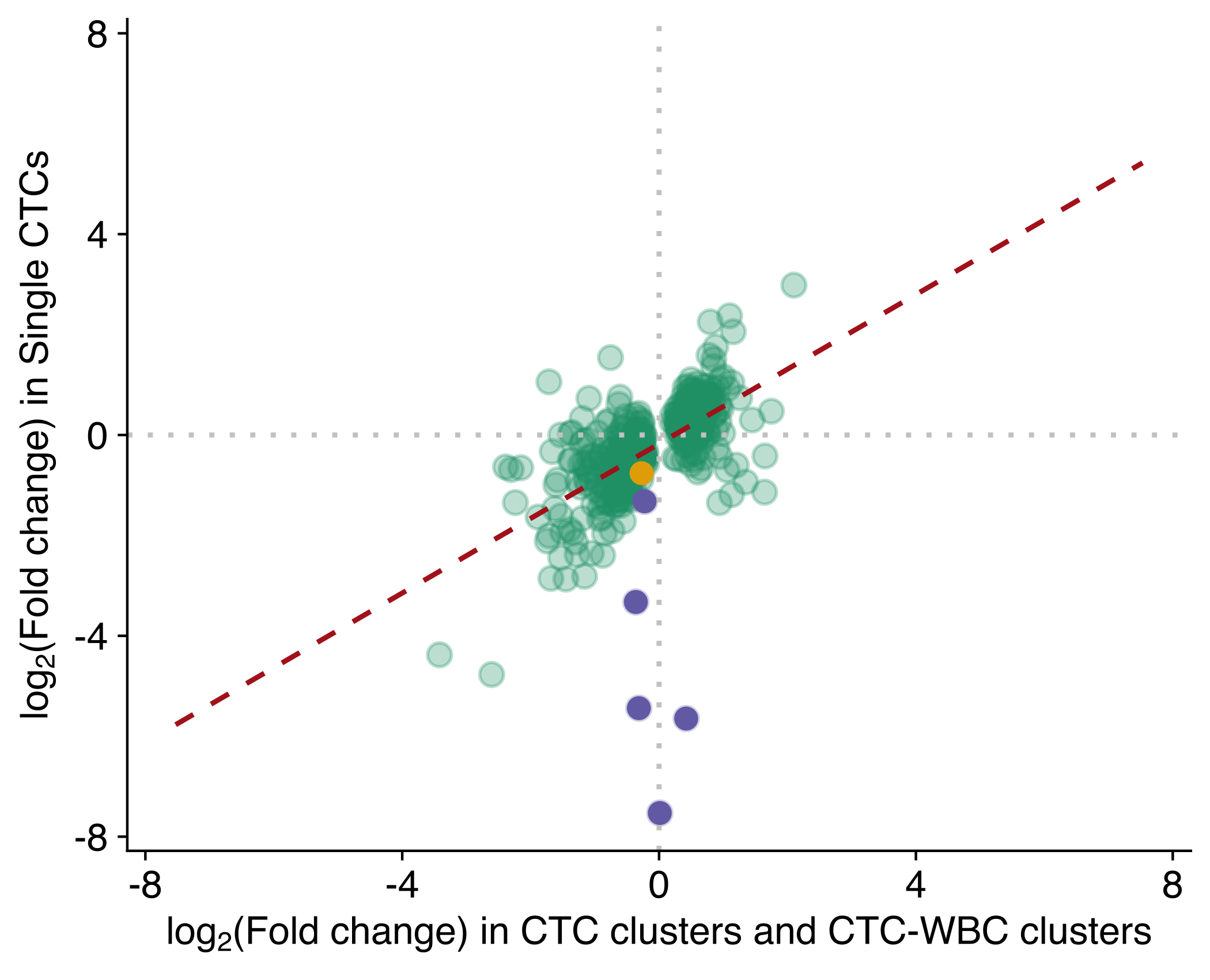
| Version | Author | Date |
|---|---|---|
| 1006c84 | fcg-bio | 2022-04-26 |
legend <- cowplot::get_legend(fc_plot_2_legend)

grid.newpage()
grid.draw(legend)
| Version | Author | Date |
|---|---|---|
| 1006c84 | fcg-bio | 2022-04-26 |
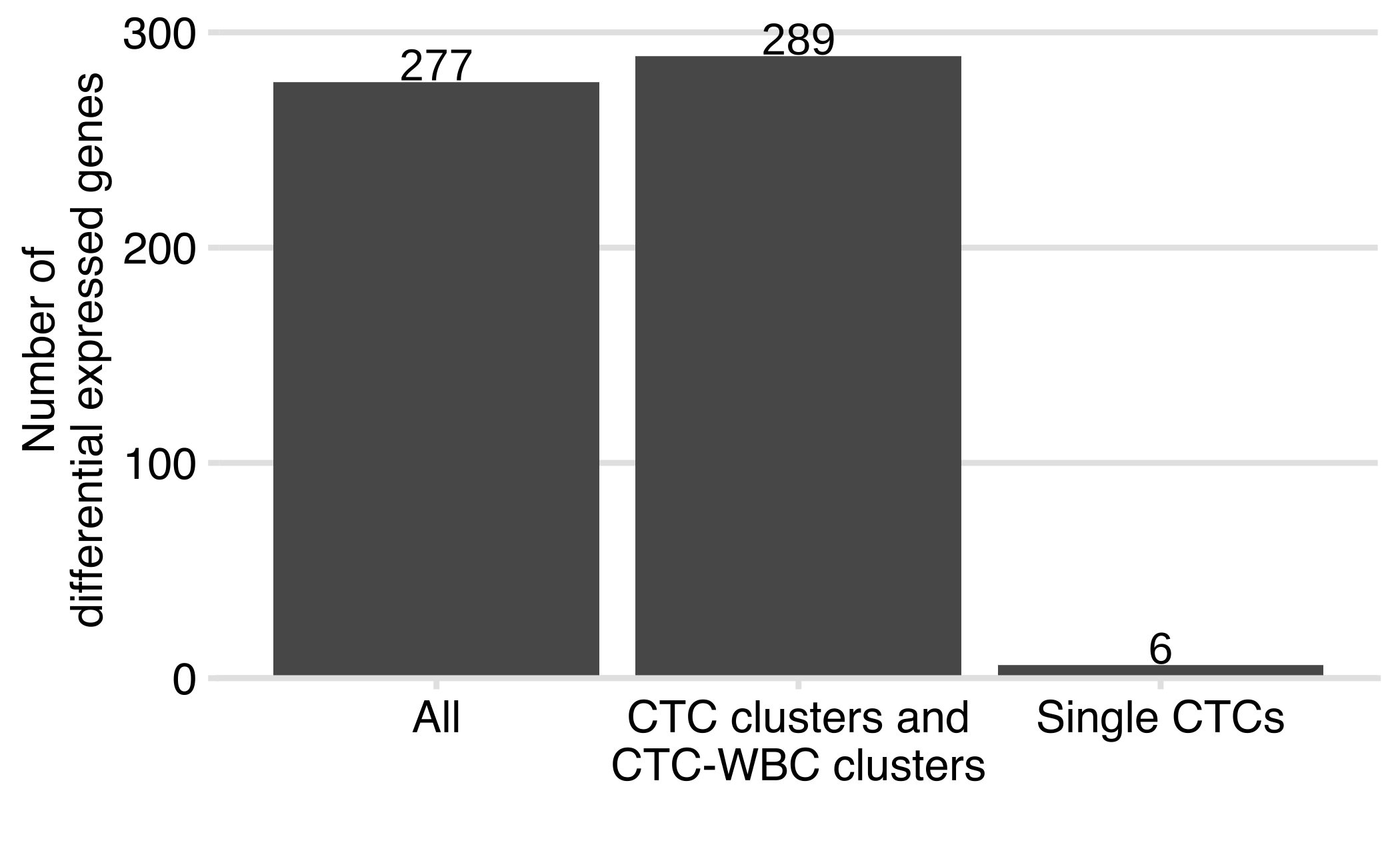
Compare DEG CTC versus CTC clusters and CTC-WBC
Bar plot showing the number of differentially expressed genes (absolute log2 fold change ≥ 0.5 and FDR ≤ 0.05) using all the samples (‘All’), using clustered CTCs (CTC clusters and CTC-WBC clusters) and using single CTCs.
results_comb <- rbind(
  dge_all$results %>% filter(FDR <= 0.05 & abs(logFC) >= 0.5) %>% mutate(sample_set = 'All'),
  dge_cluster_g$results %>% filter(FDR <= 0.05 & abs(logFC) >= 0.5) %>% mutate(sample_set = 'CTC clusters and\nCTC-WBC clusters'),
  dge_single$results %>% filter(FDR <= 0.05 & abs(logFC) >= 0.5) %>% mutate(sample_set = 'Single CTCs')
)
results_comb_Nlabels <- results_comb$sample_set %>% table %>% data.frame %>% set_names(c('sample_set', 'Freq'))

results_comb %>%
  ggplot(aes(sample_set)) +
  geom_bar() +
  ylim(c(0, 50+(results_comb_Nlabels$Freq %>% max))) +
  geom_text(aes(y=Freq, label=Freq), vjust=-0.05, color="black", size=geom_text_size, data = results_comb_Nlabels) +
  labs(
    x = '',
    y = 'Number of\ndifferential expressed genes'
  ) +
  scale_y_continuous(expand = c(0, 0), limits = c(0, 305)) +
  theme(
      panel.grid.major.y   = element_line(colour = 'grey90', size = 0.5),
      axis.ticks        = element_line(colour = 'grey90', size = 0.5),
      axis.line.x       = element_line(colour = 'grey90', size = 0.5),
      axis.line.y       = element_blank(),
    )
| Version | Author | Date |
|---|---|---|
| 1006c84 | fcg-bio | 2022-04-26 |
sessionInfo()R version 4.1.0 (2021-05-18) Platform: x86_64-apple-darwin17.0 (64-bit) Running under: macOS Big Sur 10.16
Matrix products: default BLAS: /Library/Frameworks/R.framework/Versions/4.1/Resources/lib/libRblas.dylib LAPACK: /Library/Frameworks/R.framework/Versions/4.1/Resources/lib/libRlapack.dylib
locale: [1] en_US.UTF-8/en_US.UTF-8/en_US.UTF-8/C/en_US.UTF-8/en_US.UTF-8
attached base packages: [1] grid parallel stats4 stats graphics
grDevices utils
[8] datasets methods base
other attached packages: [1] cowplot_1.1.1 DT_0.19
[3] RColorBrewer_1.1-2 circlize_0.4.13
[5] ComplexHeatmap_2.8.0 scater_1.20.1
[7] scuttle_1.2.1 SingleCellExperiment_1.14.1 [9]
SummarizedExperiment_1.22.0 Biobase_2.52.0
[11] GenomicRanges_1.44.0 GenomeInfoDb_1.28.4
[13] IRanges_2.26.0 S4Vectors_0.30.2
[15] BiocGenerics_0.38.0 MatrixGenerics_1.4.3
[17] matrixStats_0.61.0 showtext_0.9-4
[19] showtextdb_3.0 sysfonts_0.8.5
[21] forcats_0.5.1 stringr_1.4.0
[23] dplyr_1.0.7 purrr_0.3.4
[25] readr_2.0.2 tidyr_1.1.4
[27] tibble_3.1.5 ggplot2_3.3.5
[29] tidyverse_1.3.1 workflowr_1.6.2
loaded via a namespace (and not attached): [1] ggbeeswarm_0.6.0
colorspace_2.0-2
[3] rjson_0.2.20 ellipsis_0.3.2
[5] rprojroot_2.0.2 XVector_0.32.0
[7] GlobalOptions_0.1.2 BiocNeighbors_1.10.0
[9] fs_1.5.0 clue_0.3-60
[11] rstudioapi_0.13 farver_2.1.0
[13] fansi_0.5.0 lubridate_1.8.0
[15] xml2_1.3.2 splines_4.1.0
[17] codetools_0.2-18 sparseMatrixStats_1.4.2
[19] doParallel_1.0.16 knitr_1.36
[21] jsonlite_1.7.2 Cairo_1.5-12.2
[23] broom_0.7.10 cluster_2.1.2
[25] dbplyr_2.1.1 png_0.1-7
[27] compiler_4.1.0 httr_1.4.2
[29] backports_1.3.0 assertthat_0.2.1
[31] Matrix_1.3-4 fastmap_1.1.0
[33] cli_3.1.0 later_1.3.0
[35] BiocSingular_1.8.1 htmltools_0.5.2
[37] tools_4.1.0 rsvd_1.0.5
[39] gtable_0.3.0 glue_1.4.2
[41] GenomeInfoDbData_1.2.6 Rcpp_1.0.7
[43] cellranger_1.1.0 jquerylib_0.1.4
[45] vctrs_0.3.8 nlme_3.1-153
[47] crosstalk_1.1.1 iterators_1.0.13
[49] DelayedMatrixStats_1.14.3 xfun_0.27
[51] beachmat_2.8.1 rvest_1.0.2
[53] lifecycle_1.0.1 irlba_2.3.3
[55] zlibbioc_1.38.0 scales_1.1.1
[57] hms_1.1.1 promises_1.2.0.1
[59] yaml_2.2.1 gridExtra_2.3
[61] sass_0.4.0 stringi_1.7.5
[63] highr_0.9 foreach_1.5.1
[65] ScaledMatrix_1.0.0 BiocParallel_1.26.2
[67] shape_1.4.6 rlang_0.4.12
[69] pkgconfig_2.0.3 bitops_1.0-7
[71] evaluate_0.14 lattice_0.20-45
[73] labeling_0.4.2 htmlwidgets_1.5.4
[75] tidyselect_1.1.1 magrittr_2.0.1
[77] R6_2.5.1 generics_0.1.1
[79] DelayedArray_0.18.0 DBI_1.1.1
[81] mgcv_1.8-38 pillar_1.6.4
[83] haven_2.4.3 whisker_0.4
[85] withr_2.4.2 RCurl_1.98-1.5
[87] modelr_0.1.8 crayon_1.4.2
[89] utf8_1.2.2 tzdb_0.2.0
[91] rmarkdown_2.11 GetoptLong_1.0.5
[93] viridis_0.6.2 readxl_1.3.1
[95] git2r_0.28.0 reprex_2.0.1
[97] digest_0.6.28 httpuv_1.6.3
[99] munsell_0.5.0 beeswarm_0.4.0
[101] viridisLite_0.4.0 vipor_0.4.5
[103] bslib_0.3.1