Report of GSEA results for NSG-CDX-BR16, NSG-LM2 models and patient data

workflowr

• Summary
• Checks
• Past versions

Last updated: 2022-05-12

Checks: 7 0

Knit directory: diamantopoulou-ctc-dynamics/

This reproducible R Markdown analysis was created with workflowr (version 1.6.2). The Checks tab describes the reproducibility checks that were applied when the results were created. The Past versions tab lists the development history.

---

R Markdown file: up-to-date

Great! Since the R Markdown file has been committed to the Git repository, you know the exact version of the code that produced these results.

Environment: empty

Great job! The global environment was empty. Objects defined in the global environment can affect the analysis in your R Markdown file in unknown ways. For reproduciblity it’s best to always run the code in an empty environment.

Seed: set.seed(20220425)

The command set.seed(20220425) was run prior to running the code in the R Markdown file. Setting a seed ensures that any results that rely on randomness, e.g. subsampling or permutations, are reproducible.

Session information: recorded

Great job! Recording the operating system, R version, and package versions is critical for reproducibility.

Cache: none

Nice! There were no cached chunks for this analysis, so you can be confident that you successfully produced the results during this run.

File paths: relative

Great job! Using relative paths to the files within your workflowr project makes it easier to run your code on other machines.

Repository version: a747daf

Great! You are using Git for version control. Tracking code development and connecting the code version to the results is critical for reproducibility.

The results in this page were generated with repository version a747daf. See the Past versions tab to see a history of the changes made to the R Markdown and HTML files.

Note that you need to be careful to ensure that all relevant files for the analysis have been committed to Git prior to generating the results (you can use wflow_publish or wflow_git_commit). workflowr only checks the R Markdown file, but you know if there are other scripts or data files that it depends on. Below is the status of the Git repository when the results were generated:

Ignored files:
    Ignored:    .Rhistory
    Ignored:    .Rproj.user/

Untracked files:
    Untracked:  analysis/0_differential_expression_gsea_gsva.md
    Untracked:  analysis/about.md
    Untracked:  analysis/br16_dge.md
    Untracked:  analysis/br16_pca.md
    Untracked:  analysis/core_gene_sets.md
    Untracked:  analysis/gsea_across_models.md
    Untracked:  analysis/index.md
    Untracked:  analysis/license.md
    Untracked:  analysis/patients_ctc_counts_distribution.md
    Untracked:  data/differential_expression/
    Untracked:  data/patients/
    Untracked:  data/resources/
    Untracked:  data/sce/

Note that any generated files, e.g. HTML, png, CSS, etc., are not included in this status report because it is ok for generated content to have uncommitted changes.

---

These are the previous versions of the repository in which changes were made to the R Markdown (analysis/gsea_across_models.Rmd) and HTML (docs/gsea_across_models.html) files. If you’ve configured a remote Git repository (see ?wflow_git_remote), click on the hyperlinks in the table below to view the files as they were in that past version.

File	Version	Author	Date	Message
Rmd	a747daf	fcg-bio	2022-05-12	Updated legenf title
html	1fc87b5	fcg-bio	2022-05-10	Build site.
html	8fb5513	fcg-bio	2022-05-10	Build site.
html	8acaa64	fcg-bio	2022-04-26	Build site.
Rmd	545ee28	fcg-bio	2022-04-26	release v1.0
html	545ee28	fcg-bio	2022-04-26	release v1.0
html	74b1891	fcg-bio	2022-04-26	Build site.
html	c0865c6	fcg-bio	2022-04-26	Build site.
html	a136590	fcg-bio	2022-04-26	Build site.
html	bfb622b	fcg-bio	2022-04-26	Build site.
Rmd	2ef6f7f	fcg-bio	2022-04-26	added gsea and gsva tables
html	1006c84	fcg-bio	2022-04-26	Build site.
Rmd	0ded9f5	fcg-bio	2022-04-26	added final code

---

Load libraries, additional functions and data

Setup environment

knitr::opts_chunk$set(results='asis', echo=TRUE, message=FALSE, warning=FALSE, error=FALSE, fig.align = 'center', fig.width = 3.5, fig.asp = 0.618, dpi = 600, dev = c("png", "pdf"), fig.showtext = TRUE)

options(stringsAsFactors = FALSE)

Load packages

library(tidyverse)
library(showtext)
library(scater)
library(clusterProfiler)
library(enrichplot)
library(ComplexHeatmap)
library(circlize)
library(RColorBrewer)
library(cowplot)
library(DT)
library(GSVA)
library(limma)
library(colorblindr)
library(ggbeeswarm)

Set font family for figures

font_add("Helvetica", "./configuration/fonts/Helvetica.ttc")
showtext_auto()

Load ggplot theme

source("./configuration/rmarkdown/ggplot_theme.R")

Load color palettes

source("./configuration/rmarkdown/color_palettes.R")

Load functions

source('./code/R-functions/gse_report.r')
clean_msigdb_names <- function(x) x %>% gsub('REACTOME_', '', .) %>% gsub('WP_', '', .) %>% gsub('BIOCARTA_', '', .) %>% gsub('KEGG_', '', .) %>% gsub('PID_', '', .) %>% gsub('GOBP_', '', .) %>% gsub('_', ' ', .)

Load MSigDB gene sets

gmt_files_symbols <- list(
  msigdb.c2.cp = './data/resources/MSigDB/v7.4/c2.cp.v7.4.symbols.gmt',
  msigdb.c5.bp = './data/resources/MSigDB/v7.4/c5.go.bp.v7.4.symbols.gmt'
)

gmt_files_entrez <- list(
  msigdb.c2.cp = './data/resources/MSigDB/v7.4/c2.cp.v7.4.entrez.gmt',
  msigdb.c5.bp = './data/resources/MSigDB/v7.4/c5.go.bp.v7.4.entrez.gmt'
)

# combine MSigDB.C2.CP and GO:BP
msigdb.c2.cp_file <- gsub('c2.cp', 'c2.cp.c5.bp', gmt_files_symbols$msigdb.c2.cp)
if(!file.exists(msigdb.c2.cp_file)) {
  cat_cmd <- paste('cat', gmt_files_symbols$msigdb.c5.bp,  gmt_files_symbols$msigdb.c2.cp, '>',msigdb.c2.cp_file)
  system(cat_cmd)
}
gmt_files_symbols$msigdb.c2.cp.c5.bp <- msigdb.c2.cp_file

gmt_sets <- lapply(gmt_files_symbols, function(x) read.gmt(x) %>% collect %>% .[['term']] %>% levels)

Load results from differential gene expression analyses

dge_lm2 <- readRDS(file.path(params$dge_dir, 'lm2', 'dge_edgeR_QLF_robust.rds'))
dge_patient <- readRDS(file.path(params$dge_dir, 'patient', 'dge_edgeR_QLF_robust.rds'))

Load GSEA results

gse_gsea_br16 <- readRDS(file.path(params$dge_dir, 'br16', 'gse_gsea.rds'))

Load LM2 timekinetics data

sce_lm2tk <- readRDS(file.path(params$sce_dir, 'sce_lm2_tk.rds'))
gsva_lm2tk <- readRDS(file.path(params$dge_dir, 'lm2_tk', 'gsva_c2.cp.c5.bp.rds'))

NSG-CDX-BR16 GSEA results

Gene set enrichment analysis from differentially expressed genes in CTCs of NSG-CDX-BR16 mice during the rest phase versus active phase.Table listing the enriched gene sets (n = 138, adjusted P value < 0.05) in CTCs obtained in rest versus active phase from NSG-CDX-BR16 mice. The gene set enrichment analysis (GSEA) was performed using ranking genes as input, according to fold-change as shown in Supplementary table 2. P values were obtained using FGSEA method with an eps parameter of 1e^-10.

gse_gsea_br16$GSEA$msigdb.c2.cp.c5.bp@result %>% 
  filter(p.adjust < 0.05) %>% 
  dplyr::select(ID, setSize, enrichmentScore, NES, pvalue, p.adjust, leading_edge, core_enrichment) %>% 
  mutate(
    NES = round(NES, 2),
    pvalue = format.pval(pvalue, digits = 2),
    p.adjust = format.pval(p.adjust, digits = 2)
  ) %>% 
  rename(
    `Term ID` = ID,
    `Set size` = setSize,
    `Enrichment score` = enrichmentScore,
    `P value` = pvalue,
    `Adjusted P value` = p.adjust,
    `Leading edge` = leading_edge, 
    `Core enrichment` = core_enrichment
  ) %>% 
  datatable(., 
            rownames = FALSE, 
            filter = 'top', 
            caption = 'Gene set enrichment analysis from differentially expressed genes in CTCs of NSG-CDX-BR16 mice during the rest phase versus active phase.',
            extensions = 'Buttons', 
            options = list(
              dom = 'Blfrtip',
              buttons = c('csv', 'excel')
              ))

NSG-CDX-BR16 : similarity matrix for enriched gene sets

Generate the data for the similarity heatmap

use_gse_res <- gse_gsea_br16$GSEA$msigdb.c2.cp.c5.bp

# Number of terms to show
showCategoryN <- 30

# Calculate jaccard simialrity index
use_gse_res <- pairwise_termsim(use_gse_res, method = 'JC')

# Collect sim matrix for top N terms
use_terms <- use_gse_res@result %>% 
  filter(p.adjust < 0.001) %>% head(showCategoryN) %>% collect %>% .[['ID']]
use_mat <- use_gse_res@termsim[use_terms,use_terms]

# Collect results for selected terms
use_res <- use_gse_res@result[use_terms,]

# Transform matrix to symmetric
for(x in rownames(use_mat)){
  for(y in colnames(use_mat)) {
    if(x == y) {
       use_mat[x,y] <- 1
    } else {
      max_sim <- max(c(use_mat[x,y], use_mat[y,x]), na.rm = TRUE)
      use_mat[x,y] <- max_sim
      use_mat[y,x] <- max_sim
    }
  }
}

# Collect FC values for ridge plot. Values are capped at -2 and 2
gs2id <- geneInCategory(use_gse_res)[seq_len(showCategoryN)]
gs2val <- lapply(gs2id, function(id) {
        res <- use_gse_res@geneList[id]
        res <- res[!is.na(res)]
    })
gs2val_capped <- lapply(gs2val, function(x) {x[x > 2] <- 2; x[x < -2] <- -2; x} )
lt = lapply(gs2val_capped, function(x) data.frame(density(x)[c("x", "y")]))

# Save matrix for future use
br16_gsea_sim_mat <- use_mat

Generate row annotation

nes_colors <- c(
  brewer.pal(n = 7, name ="BrBG")[6],
  brewer.pal(n = 7, name ="BrBG")[2]
)

ha_row_nes = rowAnnotation(
  NES = anno_barplot(
    use_res$NES, 
    baseline = 0,
    width =  unit(1, "cm"), 
    bar_width = 0.7,
    gp = gpar(
      fill = ifelse(use_res$NES < 0 ,  nes_colors[1],  nes_colors[2]),
      col = ifelse(use_res$NES < 0 ,  nes_colors[1],  nes_colors[2])
      )
    ),
  annotation_name_gp = gpar(fontsize = 8)
  )

col_fun_nes = colorRamp2(
  seq(max(use_res$NES), min(use_res$NES), length.out = 8), 
  brewer.pal(n = 8, name ="BrBG") %>% rev)

ha_row_nes_ht = rowAnnotation(
  NES = use_res$NES,
  border = c( NES = TRUE), 
  col = list( NES = col_fun_nes),
  simple_anno_size = unit(0.8, "cm"),
  annotation_name_rot = 0,
  annotation_name_gp = gpar(fontsize = 8)
)

col_fun_pval = colorRamp2(
  seq(max(-log10(use_res$p.adjust)), -log10(0.05), length.out = 8), 
  brewer.pal(n = 8, name ="Reds") %>% rev)

ha_row_pval = rowAnnotation(
  `-log10\n(adjusted\np value)` = -log10(use_res$p.adjust),
  border = c( `-log10\n(adjusted\np value)` = TRUE), 
  col = list( `-log10\n(adjusted\np value)` = col_fun_pval),
  simple_anno_size = unit(0.8, "cm"),
  annotation_name_rot = 0,
  annotation_name_gp = gpar(fontsize = 8),
  annotation_legend_param = list(title_gp = gpar(fontsize = 8),labels_gp = gpar(fontsize = 8))
)

Similarity matrix without row names

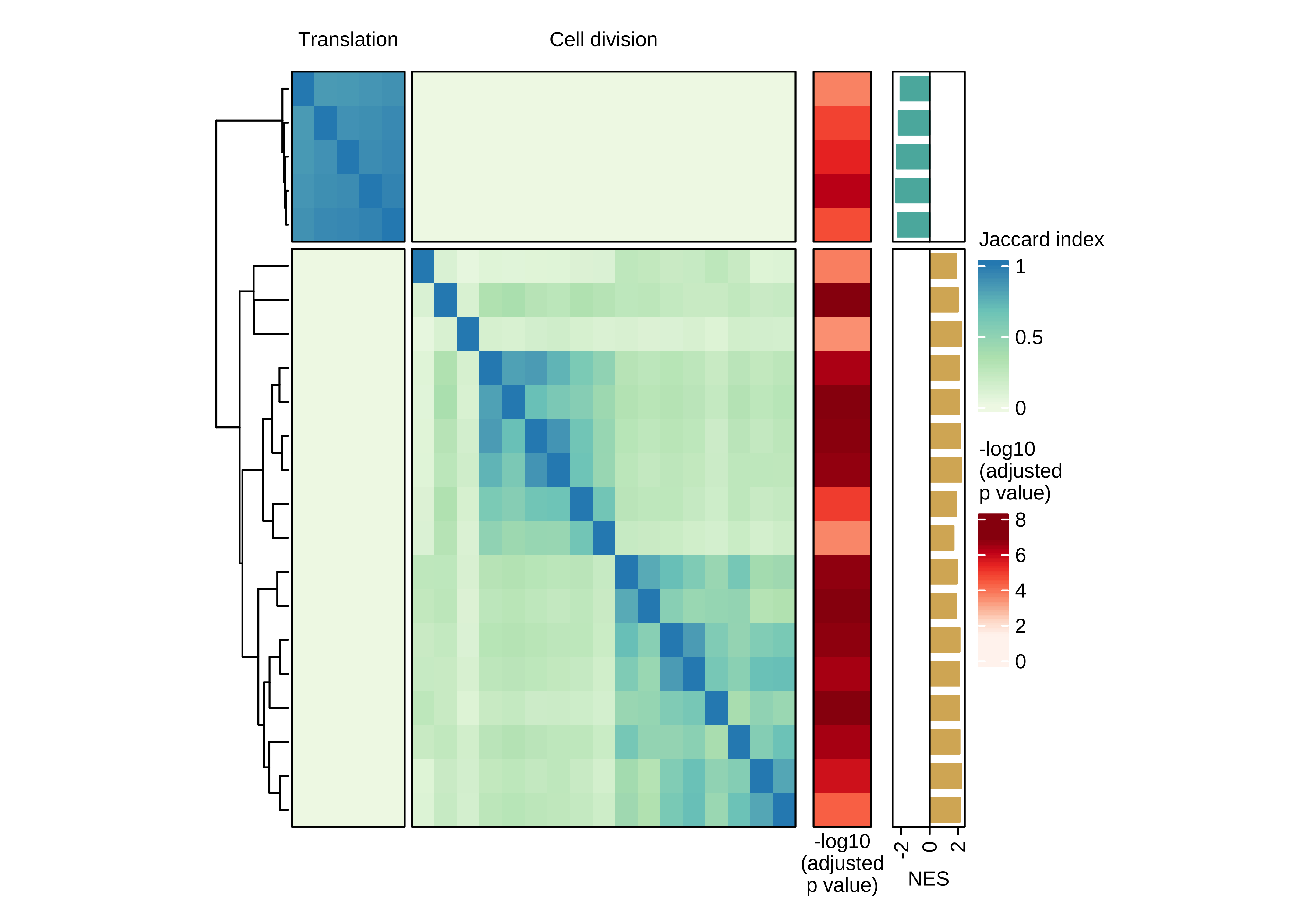
Heatmap showing the pair-wise similarity matrix of enriched gene sets (gene set enrichment analysis (GSEA), adjusted P value ≤ 0.0001) using differential expression between CTCs of rest and active phase from NSG-CDX-BR16 mice. Heatmap colors represent the Jaccard similarity coefficient. The heatmap on the right represents the adjusted P value as obtained in GSEA.

col_fun <- colorRamp2(seq(0, 1, length.out = 4), brewer.pal(4, "GnBu"))
n_split <- 2
ha_top <- HeatmapAnnotation(
  foo = anno_block(
    labels = c("Translation", "Cell division"), 
    labels_gp = gpar(col = "black", fontsize = 8),
    gp = gpar(lwd = 0, lty = 0))
  )

ht <- Heatmap(
  use_mat, 
  name = 'Jaccard index',
  column_split = n_split, 
  row_split = n_split, 
  column_title = NULL,
  row_title = NULL,
  col = col_fun,
  show_column_dend = FALSE,
  show_column_names = FALSE, 
  border = TRUE,
  top_annotation = ha_top, 
  heatmap_legend_param = list(title_gp = gpar(fontsize = 8),labels_gp = gpar(fontsize = 8)),
  width = unit(7, "cm"))

ht_br16_c2 <-  draw(ht + ha_row_pval + ha_row_nes, ht_gap = unit(c(0.2, 0.3, 0.3), "cm"))

for (slice in 1:n_split) {
  decorate_annotation("NES", {
    grid.lines(unit(c(0, 0), "native"), unit(c(0, 1), "npc"), gpar(lty = 2))
  }, slice = slice)
}

Past versions of br16_gse_heatsim_c2-1.png

Version	Author	Date
1006c84	fcg-bio	2022-04-26

cat("\n\n")

Similarity matrix with row names

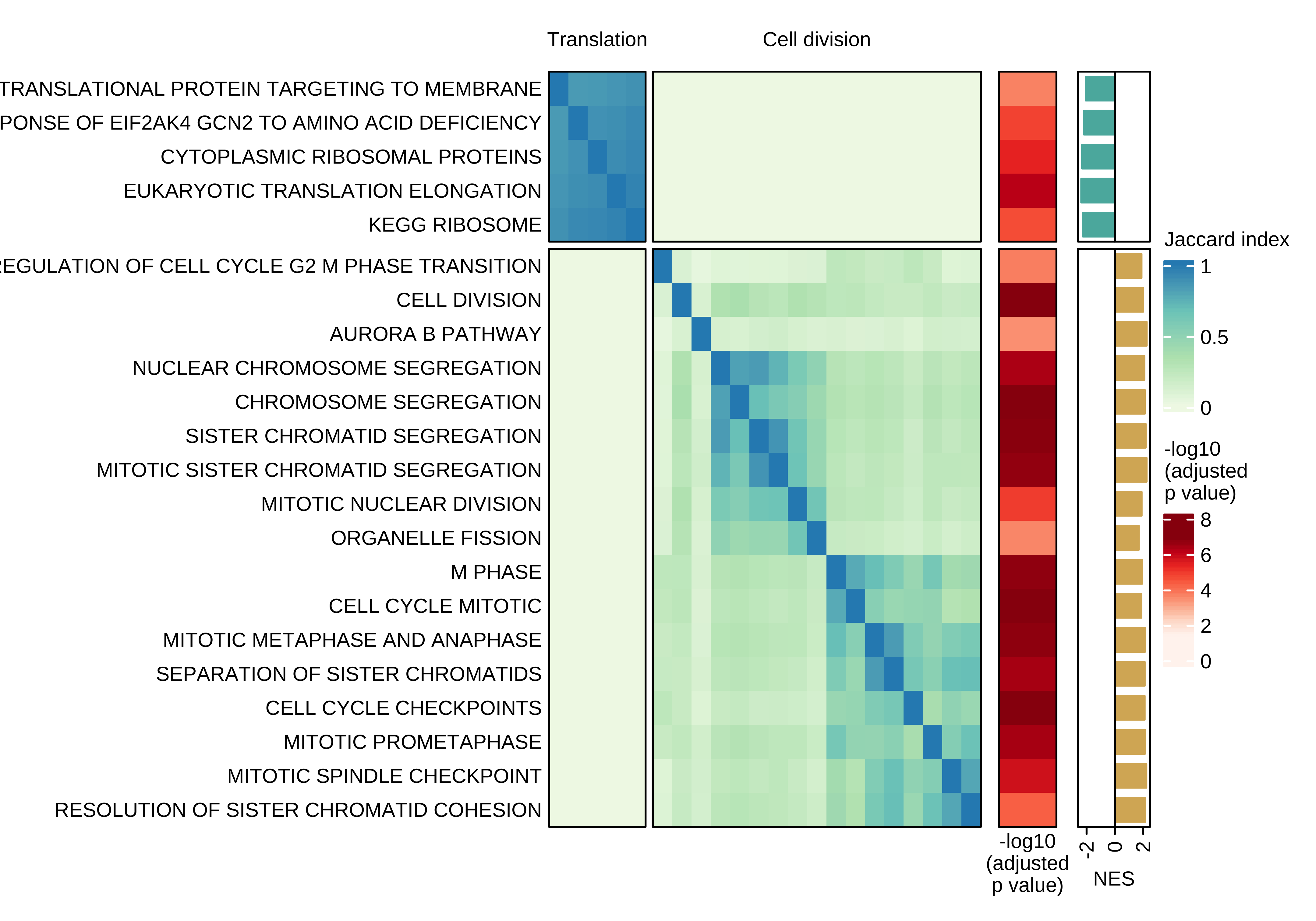
Heatmap showing the pair-wise similarity matrix of enriched gene sets (gene set enrichment analysis (GSEA), adjusted P value ≤ 0.0001) using differential expression between CTCs of rest and active phase from NSG-CDX-BR16 mice. Heatmap colors represent the Jaccard similarity coefficient. The heatmap on the right represents the adjusted P value as obtained in GSEA.

use_mat_rn <- use_mat
rownames(use_mat_rn) <- rownames(use_mat_rn) %>% 
  gsub("REACTOME_", "", .) %>% 
  gsub("BIOCARTA_", "", .) %>% 
  gsub("^PID_", "", .) %>%
  gsub("^WP_", "", .) %>%
  gsub("^PID_", "", .) %>%
  gsub("^GOBP_", "", .) %>%
  gsub("_", " ", .)

ht <- Heatmap(
  use_mat_rn, 
  name = 'Jaccard index',
  column_split = n_split, 
  row_split = n_split, 
  column_title = NULL,
  row_title = NULL,
  col = col_fun,
  show_column_dend = FALSE,
  show_column_names = FALSE, 
  show_row_dend = FALSE,
  row_names_side = "left",
  row_names_gp = gpar(fontsize = 8),
  row_names_max_width = unit(7, "cm"),
  border = TRUE,
  top_annotation = ha_top, 
  heatmap_legend_param = list(title_gp = gpar(fontsize = 8),
                              labels_gp = gpar(fontsize = 8)
                              ),
  width = unit(6, "cm"))

draw(ht + ha_row_pval + ha_row_nes, ht_gap = unit(c(0.2, 0.3, 0.3), "cm"))

for (slice in 1:n_split) {
  decorate_annotation("NES", {
    grid.lines(unit(c(0, 0), "native"), unit(c(0, 1), "npc"), gpar(lty = 2))
  }, slice = slice)
}

Past versions of br16_gse_heatsim_c2_rownames-1.png

Version	Author	Date
1006c84	fcg-bio	2022-04-26

cat("\n\n")

Save selected gsets for future use

gse_gsea_br16_f <- gse_gsea_br16$GSEA$msigdb.c2.cp.c5.bp@result %>% filter(p.adjust < 0.001)
row_order <- row_order(ht_br16_c2) %>% unlist
use_gsets <- rownames(br16_gsea_sim_mat)[row_order]
use_gmt_gsets <- read.gmt(gmt_files_symbols$msigdb.c2.cp.c5.bp)
use_gmt_gsets <- use_gmt_gsets %>% filter(term %in% use_gsets)
saveRDS(use_gsets, file = file.path(params$dge_dir, 'br16', 'ht_br16_c2_gene_sets.Rmd'))

GSEA for NSG-LM2 and Patient

Run GSEA using candidate pathways from NSG-CDX-BR16.

NSG-LM2

output_dir <- file.path(params$dge_dir, 'lm2')
dge <- dge_lm2
fc_list <- dge$results$logFC %>% set_names(dge$results$gene_name) %>% sort(decreasing = TRUE)
gsea_lm2 <- GSEA(fc_list, TERM2GENE=use_gmt_gsets, pvalueCutoff = 1)
gsea_lm2 <-  pairwise_termsim(gsea_lm2)

Patient

output_dir <- file.path(params$dge_dir, 'patient')
dge <- dge_patient
fc_list <- dge$results$logFC %>% set_names(dge$results$gene_name) %>% sort(decreasing = TRUE)
gsea_patient <- GSEA(fc_list, TERM2GENE=use_gmt_gsets, pvalueCutoff = 1)
gsea_patient <-  pairwise_termsim(gsea_patient)

Combine NSG-CDX-BR16, NSG-LM2 and patient GSEA data

gsea_lm2@result$donor <- 'LM2'
gsea_patient@result$donor <- 'Patient'
gsea_br16 <- gse_gsea_br16_f %>%
  mutate(donor = 'Br16') %>%
  dplyr::select(one_of(colnames(gsea_lm2@result)))
gsea_comb <- rbind(gsea_br16, gsea_lm2@result, gsea_patient@result)
gsea_comb <- gsea_comb %>% 
  left_join(gse_gsea_br16_f %>% dplyr::select(ID, NES, p.adjust),
            by = 'ID',
            suffix = c("", ".br16")) %>% 
  mutate(ID = factor(ID, levels = rev(use_gsets)))

Table differential expression in NSG-LM2

Genes differentially expressed in CTCs of NSG-LM26 mice during the rest phase versus active phase. Table listing the differentially expressed genes comparing CTCs obtained in the rest phase (n = 65) versus the active phase (n = 73) of NSG-CDX-BR16 mice. All genes evaluated are included in the table (n = 12,261). Fold-change and P values were computed with the quasi-likelihood (QL) approach from edgeR using robust dispersion estimates. For fold-change calculation, active phase samples were used in the denominator.

dge_lm2$results %>% 
  dplyr::select(gene_name, gene_type, logFC, logCPM, PValue, FDR, description) %>% 
  rownames_to_column('Ensemble ID') %>% 
  mutate(
    logFC = round(logFC, 2),
    logCPM = round(logCPM, 2),
    PValue = format.pval(PValue, digits = 2),
    FDR = format.pval(FDR, digits = 2),
    description = gsub(" \\[.*\\]", "", description)
  ) %>% 
  dplyr::rename(
    `Gene name` = gene_name,
    `Gene type` = gene_type
  ) %>% 
  datatable(., 
            rownames = FALSE, 
            filter = 'top', 
            caption = 'Differential expression analysis in CTCs of NSG-LM2 mice during the rest phase versus active phase.',
            extensions = 'Buttons', 
            options = list(
              dom = 'Blfrtip',
              buttons = c('csv', 'excel')
              ))

Table GSEA in NSG-LM2

Gene set enrichment analysis from gene expression in CTCs of NSG-LM2 mice during the rest phase versus active phase. Table listing the gene set enrichment results in CTCs obtained in rest versus active phase from NSG-LM2 mice. Only gene sets enriched in NSG-CDX-BR16 were analysed (n = 22, adjusted P value ≤ 0.0001). The gene set enrichment analysis (GSEA) was performed using ranked genes by fold-change as input.

gsea_lm2@result %>% 
  dplyr::select(ID, setSize, enrichmentScore, NES, pvalue, p.adjust, leading_edge, core_enrichment) %>% 
  mutate(
    NES = round(NES, 2),
    pvalue = format.pval(pvalue, digits = 2),
    p.adjust = format.pval(p.adjust, digits = 2)
  ) %>% 
  rename(
    `Term ID` = ID,
    `Set size` = setSize,
    `Enrichment score` = enrichmentScore,
    `P value` = pvalue,
    `Adjusted P value` = p.adjust,
    `Leading edge` = leading_edge, 
    `Core enrichment` = core_enrichment
  ) %>% 
  datatable(., 
            rownames = FALSE, 
            filter = 'top', 
            caption = 'Gene set enrichment analysis in CTCs of NSG-LM2 mice during the rest phase versus active phase. Only enriched gene sets from NSG-CDX-BR16 were analysed.',
            extensions = 'Buttons', 
            options = list(
              dom = 'Blfrtip',
              buttons = c('csv', 'excel')
              ))

Table differential expression in Patients

Genes differentially expressed in CTCs of breast cancer patients during the rest phase versus active phase. Table listing the differentially expressed genes comparing CTCs obtained in the rest phase (n = 65) versus the active phase (n = 73) of NSG-CDX-BR16 mice. All genes evaluated are included in the table (n = 12,261). Fold-change and P values were computed with the quasi-likelihood (QL) approach from edgeR using robust dispersion estimates. For fold-change calculation, active phase samples were used in the denominator.

dge_patient$results %>% 
  dplyr::select(gene_name, gene_type, logFC, logCPM, PValue, FDR, description) %>% 
  rownames_to_column('Ensemble ID') %>% 
  mutate(
    logFC = round(logFC, 2),
    logCPM = round(logCPM, 2),
    PValue = format.pval(PValue, digits = 2),
    FDR = format.pval(FDR, digits = 2),
    description = gsub(" \\[.*\\]", "", description)
  ) %>% 
  dplyr::rename(
    `Gene name` = gene_name,
    `Gene type` = gene_type
  ) %>% 
  datatable(., 
            rownames = FALSE, 
            filter = 'top', 
            caption = 'Differential expression analysis in CTCs of breast cancer patient during the rest phase versus active phase.',
            extensions = 'Buttons', 
            options = list(
              dom = 'Blfrtip',
              buttons = c('csv', 'excel')
              ))

Table GSEA in Patients

Gene set enrichment analysis from gene expression in CTCs of breast cancer patients during the rest phase versus active phase. Table listing the gene set enrichment results in CTCs obtained in rest versus active phase from breast cancer patients. Only gene sets enriched in NSG-CDX-BR16 were analysed (n = 22, adjusted P value ≤ 0.0001). The gene set enrichment analysis (GSEA) was performed using ranked genes by fold-change as input.

gsea_patient@result %>% 
  dplyr::select(ID, setSize, enrichmentScore, NES, pvalue, p.adjust, leading_edge, core_enrichment) %>% 
  mutate(
    NES = round(NES, 2),
    pvalue = format.pval(pvalue, digits = 2),
    p.adjust = format.pval(p.adjust, digits = 2)
  ) %>% 
  rename(
    `Term ID` = ID,
    `Set size` = setSize,
    `Enrichment score` = enrichmentScore,
    `P value` = pvalue,
    `Adjusted P value` = p.adjust,
    `Leading edge` = leading_edge, 
    `Core enrichment` = core_enrichment
  ) %>% 
  datatable(., 
            rownames = FALSE, 
            filter = 'top', 
            caption = 'Gene set enrichment analysis in CTCs of breast cancer patient during the rest phase versus active phase. Only enriched gene sets from NSG-CDX-BR16 were analysed.',
            extensions = 'Buttons', 
            options = list(
              dom = 'Blfrtip',
              buttons = c('csv', 'excel')
              ))

GSEA for NSG-CDX-BR16 and NSG-LM2

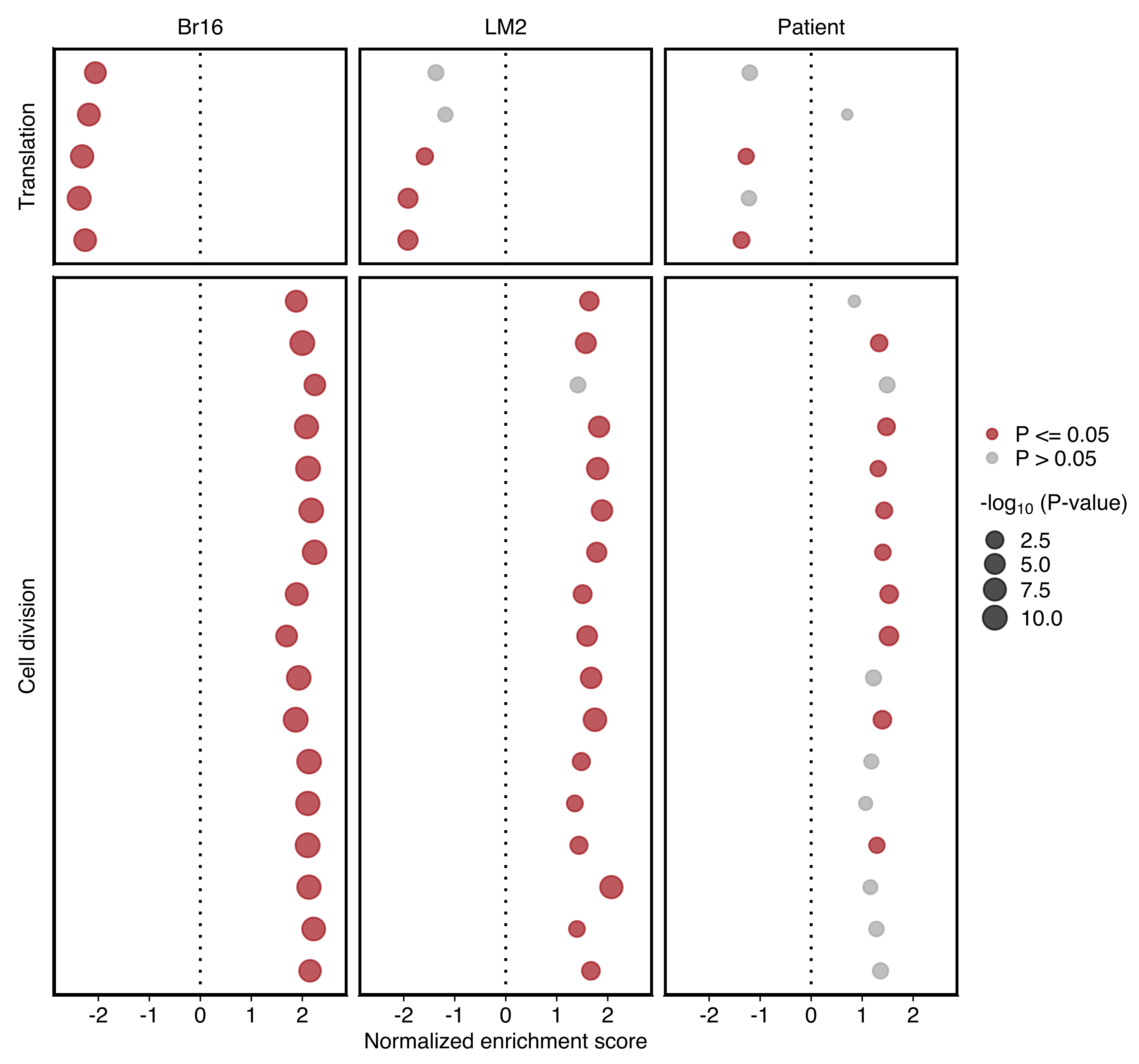
Plot comparing the normalized enrichment score (NES) and adjusted P value (dot size) obtained using GSEA for gene sets shown in “d”. Left and right panels show the results for NSG-CDX-BR16 and NSG-LM2 models, respectively. Gene sets with an adjusted P value ≤ 0.05 in each sample set are highlighted in red.

label_func <- default_labeller(18)
xlim <- (gsea_comb$NES %>% abs %>% max) + 0.25
dotplot_br16 <- gsea_comb %>% 
  filter(donor == 'Br16') %>% 
  mutate(
    color = ifelse(pvalue <= 0.05, 'P <= 0.05', 'P > 0.05'),
    row_split = ifelse(NES.br16 < 0, 'Translation', 'Cell division') %>% factor(levels=c('Translation', 'Cell division'))
    ) %>% 
  ggplot(aes(x = NES, y = ID, size = -log10(pvalue), color = color)) +
    geom_point(alpha = 0.7) +
    scale_color_manual(values = c(`P <= 0.05` = 'firebrick', `P > 0.05` = 'grey70')) +
    scale_y_discrete(labels = label_func) +
    scale_size(range = c(1.5, 3.8)) +
    labs(
      x = 'Normalized enrichment score',
      y = NULL,
      color = NULL,
      size = bquote("-log"[10] ~ .(paste0("(P-value)")))
    ) +
  facet_grid(cols = vars(donor), row = vars(row_split), scales = 'free_y', space = 'free', switch = "y") +
  xlim(c(-xlim, xlim)) +
  geom_vline(xintercept = 0, lty = 3) +
  panel_border(color = "black") +
  theme(
    axis.title.y=element_blank(),
    axis.ticks.y=element_blank(),
    axis.text.y=element_blank(),
    strip.background = element_rect(fill = 'white'),
    strip.placement = "outside"
    )

dotplot_lm2<- gsea_comb %>% 
  filter(donor == 'LM2') %>% 
  mutate(
    color = ifelse(pvalue <= 0.05, 'P <= 0.05', 'P > 0.05'),
    row_split = ifelse(NES.br16 < 0, 'Translation', 'Cell division') %>% factor(levels=c('Translation', 'Cell division'))
    ) %>% 
  ggplot(aes(x = NES, y = ID, size = -log10(pvalue), color = color)) +
    geom_point(alpha = 0.7) +
    scale_color_manual(values = c(`P <= 0.05` = 'firebrick', `P > 0.05` = 'grey70')) +
    scale_y_discrete(labels = label_func) +
    scale_size(range = c(1.5, 3.8)) +
    labs(
      x = 'Normalized enrichment score',
      y = NULL,
      color = NULL,
      size = bquote("-log"[10] ~ .(paste0("(P-value)")))
    ) +
  facet_grid(cols = vars(donor), row = vars(row_split), scales = 'free_y', space = 'free', switch = "y") +
  xlim(c(-xlim, xlim)) +
  geom_vline(xintercept = 0, lty = 3) +
  panel_border(color = "black") +
  theme(
    axis.title.y=element_blank(),
    axis.ticks.y=element_blank(),
    axis.text.y=element_blank(),
    strip.background = element_rect(fill = 'white'),
    strip.placement = "outside"
    )

plot_grid(dotplot_br16, dotplot_lm2)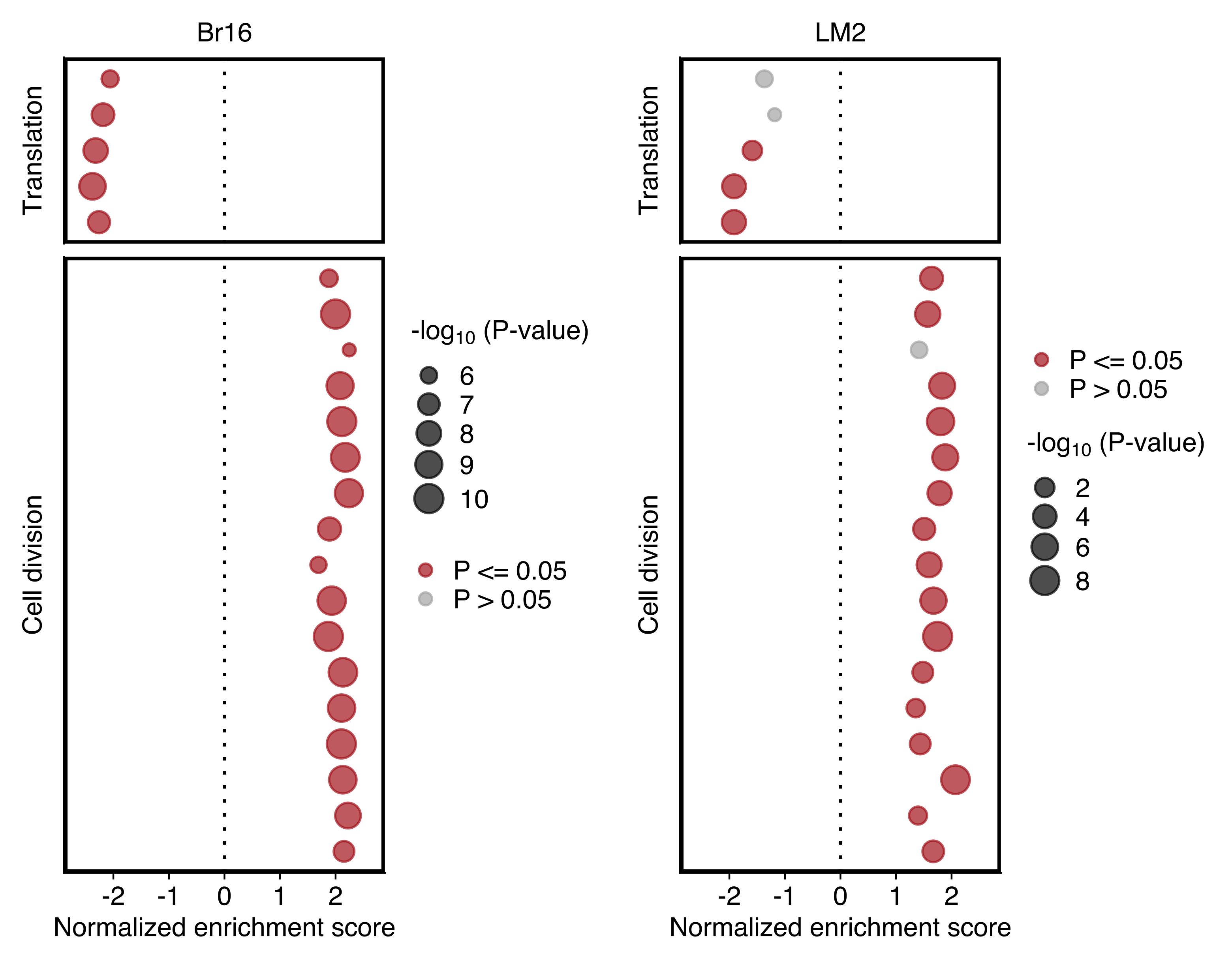

Past versions of br16_lm2_nes_dotplot_c2-1.png

Version	Author	Date
1006c84	fcg-bio	2022-04-26

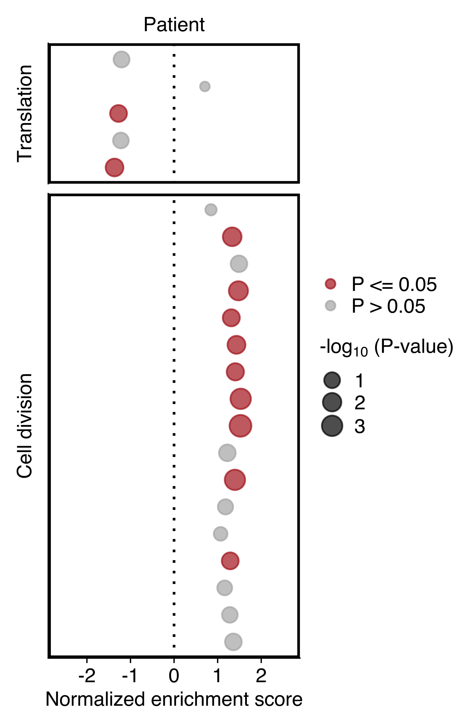
GSEA for Patient

Plot showing the NES and P value (dot size) in patient CTCs obtained using GSEA for gene sets shown in “d”. Gene sets with an P value ≤ 0.05 are highlighted in red (bottom).

label_func <- default_labeller(18)
xlim <- (gsea_comb$NES %>% abs %>% max) + 0.25
gsea_comb %>% 
  filter(donor == 'Patient') %>% 
  mutate(
    color = ifelse(pvalue <= 0.05, 'P <= 0.05', 'P > 0.05'),
    row_split = ifelse(NES.br16 < 0, 'Translation', 'Cell division') %>% factor(levels=c('Translation', 'Cell division'))
    ) %>% 
  ggplot(aes(x = NES, y = ID, size = -log10(pvalue), color = color)) +
    geom_point(alpha = 0.7) +
    scale_color_manual(values = c(`P <= 0.05` = 'firebrick', `P > 0.05` = 'grey70')) +
    scale_y_discrete(labels = label_func) +
    scale_size(range = c(1.5, 3.8)) +
    labs(
      x = 'Normalized enrichment score',
      y = NULL,
      color = NULL,
      size = bquote("-log"[10] ~ .(paste0("(P-value)")))
    ) +
  facet_grid(cols = vars(donor), row = vars(row_split), scales = 'free_y', space = 'free', switch = "y") +
  xlim(c(-xlim, xlim)) +
  geom_vline(xintercept = 0, lty = 3) +
  panel_border(color = "black") +
  theme(
    axis.title.y=element_blank(),
    axis.ticks.y=element_blank(),
    axis.text.y=element_blank(),
    strip.background = element_rect(fill = 'white'),
    strip.placement = "outside"
    )

Past versions of patient_nes_dotplot_c2-1.png

Version	Author	Date
1006c84	fcg-bio	2022-04-26

GSEA for NSG-CDX-BR16, NSG-LM2 and patient

Plots comparing the normalized enrichment score (NES) and adjusted P value (dot size) obtained using GSEA for gene sets shown in “d”. Gene sets with an adjusted P value ≤ 0.05 in each sample set are highlighted in red

label_func <- default_labeller(18)
xlim <- (gsea_comb$NES %>% abs %>% max) + 0.25
gsea_comb %>% 
  mutate(
    color = ifelse(pvalue <= 0.05, 'P <= 0.05', 'P > 0.05'),
    row_split = ifelse(NES.br16 < 0, 'Translation', 'Cell division') %>% factor(levels=c('Translation', 'Cell division'))
    ) %>% 
  ggplot(aes(x = NES, y = ID, size = -log10(pvalue), color = color)) +
    geom_point(alpha = 0.7) +
    scale_color_manual(values = c(`P <= 0.05` = 'firebrick', `P > 0.05` = 'grey70')) +
    scale_y_discrete(labels = label_func) +
    scale_size(range = c(1.5, 3.8)) +
    labs(
      x = 'Normalized enrichment score',
      y = NULL,
      color = NULL,
      size = bquote("-log"[10] ~ .(paste0("(P-value)")))
    ) +
  facet_grid(cols = vars(donor), row = vars(row_split), scales = 'free_y', space = 'free', switch = "y") +
  xlim(c(-xlim, xlim)) +
  geom_vline(xintercept = 0, lty = 3) +
  panel_border(color = "black") +
  theme(
    axis.title.y=element_blank(),
    axis.ticks.y=element_blank(),
    axis.text.y=element_blank(),
    strip.background = element_rect(fill = 'white'),
    strip.placement = "outside"
    )

Past versions of br16_lm2_patient_nes_dotplot-1.png

Version	Author	Date
1006c84	fcg-bio	2022-04-26

GSVA for NSG-LM2

Run differential expression

Run differential expression at pathway level removing timepoint 0600 (ZT = 0, only 1 biological replicate) and using only candidate pathways from BR16 analysis. We use limma (Smyth 2004) as suggested in GSVA vignette. For several groups (timepoints) we are using the strategy defined at limma vignette Section 9.3

use_sce <- sce_lm2tk
gsva_res <- gsva_lm2tk
use_gsets_nes <-  gse_gsea_br16$GSEA$msigdb.c2.cp.c5.bp@result[use_gsets, 'NES'] %>% set_names(use_gsets)
use_gsets_cat <- ifelse(use_gsets_nes < 0, 'Translation', 'Cell division') %>% factor(levels=c('Translation', 'Cell division'))
use_gmt_gsets <- read.gmt(gmt_files_symbols$msigdb.c2.cp.c5.bp)
use_gmt_gsets <- use_gmt_gsets %>% filter(term %in% use_gsets)

# Remove 06000 samples, only one replicate
use_samples <- intersect(colnames(gsva_res), use_sce[,use_sce$timepoint!='0600']$sample_alias)

# limma
f <- use_sce[,use_samples]$timepoint %>% factor
design <- model.matrix(~ 0 + f)
gsva_res_sel <- gsva_res[use_gsets,use_samples]
fit <- lmFit(gsva_res_sel, design)
contrast_to_eval <- combn(colnames(design), 2, simplify = TRUE) %>% apply(., 2, function(x) paste(x, collapse = '-'))
contrast.matrix <- makeContrasts(contrasts = contrast_to_eval, levels = colnames(design))                                  
fit2 <- contrasts.fit(fit, contrast.matrix)
fit2 <- eBayes(fit2)

limma_res <- topTable(fit2, number=100000) %>% 
  rownames_to_column('Term') %>% 
  mutate(to_rownames = Term) %>% 
  column_to_rownames('to_rownames')
limma_res$Term_cat <- use_gsets_cat[limma_res$Term]

Additional objects for plotting

coldata_ord <- colData(use_sce) %>% data.frame %>% arrange(zt, sample_type)
gsva_mat <- gsva_res[use_gsets, coldata_ord$sample_alias]
gsva_df <- gsva_mat %>% data.frame %>% 
  rownames_to_column('term') %>% 
  pivot_longer(-term, names_to = 'sample_alias') %>% 
  left_join(coldata_ord) %>% 
  mutate(term = factor(term, levels = use_gsets))
gsva_df$term_cat <- use_gsets_cat[gsva_df$term]

gsva_avg_df <- gsva_df %>%
  group_by(zt, timepoint, term) %>% 
  summarise(mean_gsva = mean(value)) %>% 
  mutate(term = factor(term, levels = use_gsets))
gsva_avg_df$term_cat <- use_gsets_cat[gsva_avg_df$term]

gsva_df$term <- clean_msigdb_names(gsva_df$term) %>% factor(., clean_msigdb_names(use_gsets))
gsva_avg_df$term <- clean_msigdb_names(gsva_avg_df$term) %>% factor(., clean_msigdb_names(use_gsets))

gsva_avg_mat <- gsva_avg_df %>% 
  ungroup() %>% 
  dplyr::select(-term_cat, -timepoint) %>% 
  pivot_wider(names_from = zt, values_from = mean_gsva) %>% 
  column_to_rownames('term') %>% 
  as.matrix

gsva_avg_mat <- gsva_avg_mat[clean_msigdb_names(use_gsets),]

GSVA table of results

Gene set variation analysis in CTCs of theNSG-LM2 time-kinetics experiment. Table listing the results from the differential analysis of gene set variation analysis (GSVA) scores in CTC of the NSG-LM2 time-kinetics experiment. Only gene sets enriched in NSG-CDX-BR16 were analysed (n = 22, adjusted P value ≤ 0.0001). The F statistic and the corresponding P value generated by limma, combine the pair-wise comparisons between all the time points in the experiment with more than three replicates (n = 6 comparisons). GSVA scores for each individual sample are listed at the end of the table.

gsva_res_sel %>% 
  as.data.frame %>% 
  rownames_to_column('Term') %>% 
  left_join(limma_res) %>% 
  mutate(
    P.Value = format.pval(P.Value, digits = 2),
    adj.P.Val = format.pval(adj.P.Val, digits = 2)
  ) %>% 
  dplyr::select(Term, Term_cat,AveExpr:adj.P.Val, LM2_Clusters_0200_1:LM2_WBC_2200_1) %>% 
  rename(
    `Term ID` = Term,
    `Category` = Term_cat,
    `Average GSVA score` = AveExpr,
    `P value` = P.Value,
    `Adjusted P value` = adj.P.Val,
  ) %>% 
  datatable(., 
            rownames = FALSE, 
            filter = 'top', 
            caption = 'Results from differential enrichment across timepoints of NSG-LM2 time kinetics experiment. Only enriched gene sets from NSG-CDX-BR16 were reported. The F statistic and the corresponding P value combine the pair-wise comparisons between all the time points in the experiment with more than three replicates. GSVA scores for each individual sample are listed at the end of the table.',
            extensions = 'Buttons', 
            options = list(
              dom = 'Blfrtip',
              buttons = c('csv', 'excel')
              ))

GSVA across time series

GSVA score for translation (yellow, n= 5) and cell division (blue, n= 17) gene sets in CTCs obtained from the NSG-LM2 time-kinetics experiment. Yellow and blue lines represent the average at each time point. Individual points represent the enrichment score for each CTC sample. The white and grey backgrounds represent environmental light (rest period) and dark conditions (active period), respectively. Differential expression adjusted P values as obtained from limma are shown for each individual gene set.

bg_color <- data.frame(
  xmin = c(-2, 0, 12),
  xmax = c(0, 12, 22),
  fill_bg = c('night', 'day', 'night')
)

adj_p_df <- limma_res %>% 
  mutate(
    term = clean_msigdb_names(limma_res$Term) %>% factor(., clean_msigdb_names(use_gsets)),
    label = format.pval(adj.P.Val, digits = 1),
    label = paste("italic('P=')~", label),
    ypos = ifelse(Term_cat == 'Translation', -0.45, 0.45)
  )


ggplot() +
  geom_rect(data = bg_color, aes(xmin = xmin, xmax = xmax, ymin = -Inf, ymax = Inf, fill = fill_bg), alpha = 0.5) +
  geom_hline(yintercept = 0, lty = 2, size = 0.2) +
  geom_quasirandom(data = gsva_df, aes(zt, value, group = term, color = term_cat), size = 1, pch = 16, alpha = 0.4, width = 0.3) +
  geom_line(data = gsva_avg_df, aes(zt, mean_gsva, group = term, color = term_cat), size = 0.6, alpha = 1) +
  facet_wrap(~term, labeller = label_wrap_gen(width = 25), ncol = 5, scales = 'free_x') +
  scale_fill_manual(values = c('night' = "grey80", 'day' = "white")) +
  scale_color_OkabeIto() +
  labs(
      x = 'Time (ZT)',
      y = 'GSVA enrichment score',
      color = NULL,
      fill = NULL
    ) +
  guides(fill = FALSE) +
  scale_x_continuous(
    expand = c(0,0),
    breaks=c(0, 4, 12, 16, 20)
  ) +
  scale_y_continuous(
    expand = c(0,0),
    limits = c(-0.55, 0.55)
  ) +
  theme(
    legend.position="top",
    plot.margin = margin(14, 7, 3, 1.5),
    strip.background = element_rect(fill = 'white'),
    strip.text = element_text(size = 6)
  ) +
  geom_text(x = 16, aes(label = label, y = ypos), data = adj_p_df, size = 1.8, hjust = 0, parse = TRUE)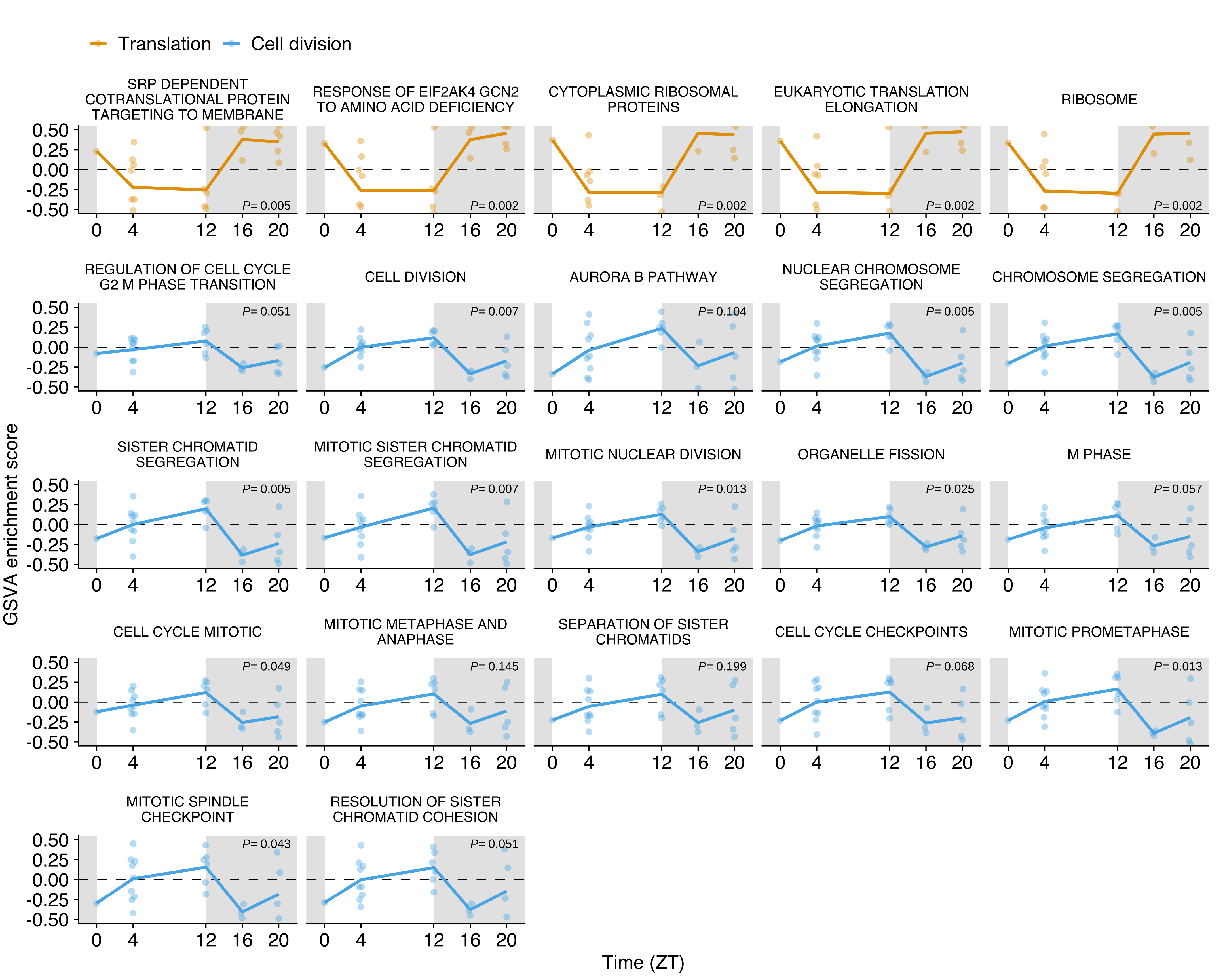

Past versions of lm2_s1_gsva_timeseries_facet_5tp-1.png

Version	Author	Date
1006c84	fcg-bio	2022-04-26

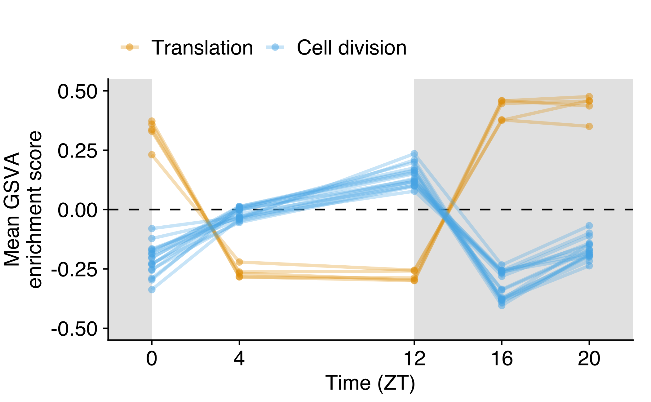
Average GSVA score across time series

Average GSVA score for translation (yellow, n=5) and cell division (blue, n=17) gene sets in CTCs obtained in the NSG-LM2 time-kinetics experiment. The average was calculated for each gene set and time point across all CTC samples (ZT0 n=1, ZT4 n=9, ZT12 n=6, ZT16 n=3, ZT20 n=5). The white and grey backgrounds represent environmental light (rest period) and dark conditions (active period), respectively.

bg_color <- data.frame(
  xmin = c(-2, 0, 12),
  xmax = c(0, 12, 22),
  fill_bg = c('night', 'day', 'night')
)

ggplot() +
  geom_rect(data = bg_color, aes(xmin = xmin, xmax = xmax, ymin = -Inf, ymax = Inf, fill = fill_bg), alpha = 0.5) +
  geom_hline(yintercept = 0, lty = 2, size = 0.3) +
  geom_line(data = gsva_avg_df, aes(zt, mean_gsva, group = term, color = term_cat), size = 0.6, alpha = 0.3) +
  geom_point(data = gsva_avg_df, aes(zt, mean_gsva, group = term, color = term_cat), size = 1, pch = 16, alpha = 0.5) +
  scale_fill_manual(values = c('night' = "grey80", 'day' = "white")) +
  scale_color_OkabeIto() +
  labs(
      x = 'Time (ZT)',
      y = 'Mean GSVA\nenrichment score',
      color = NULL,
      fill = NULL
    ) +
  guides(fill = "none") +
  scale_x_continuous(
    expand = c(0,0),
    breaks=c(0, 4, 12, 16, 20)
  ) +
  scale_y_continuous(
    expand = c(0,0),
    limits = c(-0.55, 0.55)
  ) +
  theme(
    legend.position="top",
    plot.margin = margin(14, 7, 3, 1.5)
  )

Past versions of lm2_tk_gsva_timeseries_avg-1.png

Version	Author	Date
1006c84	fcg-bio	2022-04-26

Session information

sessionInfo()

R version 4.1.0 (2021-05-18) Platform: x86_64-apple-darwin17.0 (64-bit) Running under: macOS Big Sur 10.16

Matrix products: default BLAS: /Library/Frameworks/R.framework/Versions/4.1/Resources/lib/libRblas.dylib LAPACK: /Library/Frameworks/R.framework/Versions/4.1/Resources/lib/libRlapack.dylib

locale: [1] en_US.UTF-8/en_US.UTF-8/en_US.UTF-8/C/en_US.UTF-8/en_US.UTF-8

attached base packages: [1] grid parallel stats4 stats graphics grDevices utils
[8] datasets methods base

other attached packages: [1] ggbeeswarm_0.6.0 colorblindr_0.1.0
[3] colorspace_2.0-2 limma_3.48.3
[5] GSVA_1.40.1 DT_0.19
[7] cowplot_1.1.1 RColorBrewer_1.1-2
[9] circlize_0.4.13 ComplexHeatmap_2.8.0
[11] enrichplot_1.12.3 clusterProfiler_4.0.5
[13] scater_1.20.1 scuttle_1.2.1
[15] SingleCellExperiment_1.14.1 SummarizedExperiment_1.22.0 [17] Biobase_2.52.0 GenomicRanges_1.44.0
[19] GenomeInfoDb_1.28.4 IRanges_2.26.0
[21] S4Vectors_0.30.2 BiocGenerics_0.38.0
[23] MatrixGenerics_1.4.3 matrixStats_0.61.0
[25] showtext_0.9-4 showtextdb_3.0
[27] sysfonts_0.8.5 forcats_0.5.1
[29] stringr_1.4.0 dplyr_1.0.7
[31] purrr_0.3.4 readr_2.0.2
[33] tidyr_1.1.4 tibble_3.1.5
[35] ggplot2_3.3.5 tidyverse_1.3.1
[37] workflowr_1.6.2

loaded via a namespace (and not attached): [1] utf8_1.2.2 tidyselect_1.1.1
[3] htmlwidgets_1.5.4 RSQLite_2.2.8
[5] AnnotationDbi_1.54.1 BiocParallel_1.26.2
[7] scatterpie_0.1.7 munsell_0.5.0
[9] ScaledMatrix_1.0.0 codetools_0.2-18
[11] withr_2.4.2 GOSemSim_2.18.1
[13] highr_0.9 knitr_1.36
[15] rstudioapi_0.13 DOSE_3.18.3
[17] labeling_0.4.2 git2r_0.28.0
[19] GenomeInfoDbData_1.2.6 polyclip_1.10-0
[21] bit64_4.0.5 farver_2.1.0
[23] rhdf5_2.36.0 rprojroot_2.0.2
[25] downloader_0.4 vctrs_0.3.8
[27] treeio_1.16.2 generics_0.1.1
[29] xfun_0.27 R6_2.5.1
[31] doParallel_1.0.16 clue_0.3-60
[33] graphlayouts_0.7.1 rsvd_1.0.5
[35] rhdf5filters_1.4.0 bitops_1.0-7
[37] cachem_1.0.6 fgsea_1.18.0
[39] gridGraphics_0.5-1 DelayedArray_0.18.0
[41] assertthat_0.2.1 promises_1.2.0.1
[43] scales_1.1.1 ggraph_2.0.5
[45] beeswarm_0.4.0 gtable_0.3.0
[47] beachmat_2.8.1 Cairo_1.5-12.2
[49] tidygraph_1.2.0 rlang_0.4.12
[51] GlobalOptions_0.1.2 splines_4.1.0
[53] lazyeval_0.2.2 broom_0.7.10
[55] yaml_2.2.1 reshape2_1.4.4
[57] modelr_0.1.8 crosstalk_1.1.1
[59] backports_1.3.0 httpuv_1.6.3
[61] qvalue_2.24.0 tools_4.1.0
[63] ggplotify_0.1.0 ellipsis_0.3.2
[65] jquerylib_0.1.4 Rcpp_1.0.7
[67] plyr_1.8.6 sparseMatrixStats_1.4.2
[69] zlibbioc_1.38.0 RCurl_1.98-1.5
[71] GetoptLong_1.0.5 viridis_0.6.2
[73] cluster_2.1.2 haven_2.4.3
[75] ggrepel_0.9.1 fs_1.5.0
[77] magrittr_2.0.1 data.table_1.14.2
[79] DO.db_2.9 reprex_2.0.1
[81] whisker_0.4 xtable_1.8-4
[83] hms_1.1.1 patchwork_1.1.1
[85] evaluate_0.14 XML_3.99-0.8
[87] readxl_1.3.1 shape_1.4.6
[89] gridExtra_2.3 compiler_4.1.0
[91] crayon_1.4.2 shadowtext_0.0.9
[93] htmltools_0.5.2 ggfun_0.0.4
[95] later_1.3.0 tzdb_0.2.0
[97] aplot_0.1.1 lubridate_1.8.0
[99] DBI_1.1.1 tweenr_1.0.2
[101] dbplyr_2.1.1 MASS_7.3-54
[103] Matrix_1.3-4 cli_3.1.0
[105] igraph_1.2.7 pkgconfig_2.0.3
[107] xml2_1.3.2 foreach_1.5.1
[109] annotate_1.70.0 ggtree_3.0.4
[111] vipor_0.4.5 bslib_0.3.1
[113] XVector_0.32.0 rvest_1.0.2
[115] yulab.utils_0.0.4 digest_0.6.28
[117] graph_1.70.0 Biostrings_2.60.2
[119] rmarkdown_2.11 cellranger_1.1.0
[121] fastmatch_1.1-3 tidytree_0.3.5
[123] GSEABase_1.54.0 DelayedMatrixStats_1.14.3 [125] rjson_0.2.20 lifecycle_1.0.1
[127] nlme_3.1-153 jsonlite_1.7.2
[129] Rhdf5lib_1.14.2 BiocNeighbors_1.10.0
[131] viridisLite_0.4.0 fansi_0.5.0
[133] pillar_1.6.4 lattice_0.20-45
[135] KEGGREST_1.32.0 fastmap_1.1.0
[137] httr_1.4.2 GO.db_3.13.0
[139] glue_1.4.2 png_0.1-7
[141] iterators_1.0.13 bit_4.0.4
[143] HDF5Array_1.20.0 ggforce_0.3.3
[145] stringi_1.7.5 sass_0.4.0
[147] blob_1.2.2 BiocSingular_1.8.1
[149] memoise_2.0.0 irlba_2.3.3
[151] ape_5.5